Gender Portrayal in Children's Books
We have read to our daughter every night from a young age. As soon as she was able to speak, she was asking for more books (“One more” is still her favorite phrase in any situation). One book turned into two. Two turned into three. Once we got to four books, we had to put our foot down…mostly. Some nights might creep to five.
Background
I have a book buying problem. I buy them faster than I can read. Now that I have a daughter, I can spend some of that effort on buying her books. Luckily we can read her books faster than mine, and none go unread.
We try to make sure she is reading enough books with positive female role models, and we aim to give her a diverse set of reading materials (we will see below if we were successful in that in this sample). But I was curious if the gender portrayal differed in her books.
Are we balancing the genders of the main characters? Are we reading books with diverse characters? Do books differ in sentiment depending on the gender of the main character?
Data Collection
Three types of data were collected.
-
Reading Log: Each time we read a book to our daughter, I tracked the book and whether it was read during the day or during bedtime.
-
Book Details: For each book, I tracked whether the characters were human or animal, the gender of the main character, the race of the main character, and the gender of the author. Genders were identified by the use of pronouns. While genders were not restricted to female and male, the books in this sample were limited to female, male, more than one gender, and not applicable.
-
Book Text: Using Optical Character Recognition software, I began by scanning every book, but this became too burdensome. Since I was interested in gender portrayal in these books, I quickly changed my strategy to only scanning books were there was a single gender main character. In the end, I scanned 26 of the 41 books, including 9 with human male main character and 13 with human female main character.
Analysis
While there are several packages available for textual analysis in R, here I will focus on tidytext.
library(readtext)
library(tidytext)
library(tidyverse)
Unlike other blog entries, I am not able to provide all of the data, as it contains copyrighted text. There are other options for textual analysis using books in the public domain, such as the janeaustinr package. The reading log and book details, however, are available on Github.
# book_text <- readtext("text/*.txt",
#                       docvarsfrom = "filenames",
#                       docvarnames = c("title", "year"),
#                       dvsep = "_",
#                       encoding = "UTF-8")

reading_log <- read.csv("https://raw.githubusercontent.com/bnlsn/blog-data/main/lila-book-analysis/reading-log.csv")

book_details <- read.csv("https://raw.githubusercontent.com/bnlsn/blog-data/main/lila-book-analysis/book-details.csv")

head(reading_log, 5) %>%
  knitr::kable()
| date | title | day_night |
|---|---|---|
| 1/1/2022 | Caps for Sale | Day |
| 1/1/2022 | Caps for Sale and the Mindful Monkeys | Day |
| 1/1/2022 | Bluey - The Beach | Night |
| 1/1/2022 | Bunheads | Night |
| 1/1/2022 | Flying High The Story of Gymnastics Champion Simone Biles | Night |
Each book can be read more than once, and this is indicated in the reading log. In addition to understanding how the corpus of books looks overall, we can add the number of times read to our book_details table.
Moving forward, the number of books weighted by the number of times read will be called exposure.
We can count the number of times a book appears on the reading log and join this with our book details table.
times_read <- reading_log %>%
  group_by(title) %>%
  summarise(count = n())

book_details <- left_join(book_details, times_read)

head(book_details, 5) %>%
  knitr::kable()
| title | species | main_gender | main_race | author_gender | count |
|---|---|---|---|---|---|
| Bluey - The Beach | Animal | Female | Not applicable | Unknown | 4 |
| Bunheads | Human | Female | Black or African American | Female | 4 |
| Caps for Sale | Human | Male | White | Female | 1 |
| Caps for Sale and the Mindful Monkeys | Human | Male | White | Female | 1 |
| Celtic Tales - The Giant’s Stairs | Human | Male | White | Unknown | 1 |
Book Characteristics
The summary table will include four characteristics of the books: author gender, main character gender, main character race, and main character species (human or animal). We will want to display these statistics for the set of books we read, but also for the exposure, which factors in the number of times each book was read.
Our first category is author gender. After grouping by the gender and the count of times read, we can sum up the distinct titles for our count of books, and sum up the count of times read for our exposure.
author_gender_table <- book_details %>%
  group_by(author_gender, count) %>%
  summarise(book_count = n_distinct(title), weighted.count = sum(count))
Once we have calculated the count and exposure, we will add percentages for book the book count and the exposure count.
author_gender_table <- author_gender_table %>%
  group_by(author_gender) %>%
  summarise(book_count = sum(book_count), count.pct = book_count/(sum(author_gender_table$book_count)), weighted.count = sum(weighted.count), weighted.pct = weighted.count/(sum(author_gender_table$weighted.count))) %>%
  rename(subcategory = author_gender)
author_gender_table$category = "Author Gender"
Now we can repeat this for each of our three remaining categories of information.
main_gender_table <- book_details %>%
  group_by(main_gender, count) %>%
  summarise(book_count = n_distinct(title), weighted.count = sum(count))
main_gender_table <- main_gender_table %>%
  group_by(main_gender) %>%
  summarise(book_count = sum(book_count), count.pct = book_count/(sum(main_gender_table$book_count)), weighted.count = sum(weighted.count), weighted.pct = weighted.count/(sum(main_gender_table$weighted.count))) %>%
  rename(subcategory = main_gender)
main_gender_table$category = "Main Character Gender"

main_race_table <- book_details %>%
  group_by(main_race, count) %>%
  summarise(book_count = n_distinct(title), weighted.count = sum(count))
main_race_table <- main_race_table %>%
  group_by(main_race) %>%
  summarise(book_count = sum(book_count), count.pct = book_count/(sum(main_race_table$book_count)), weighted.count = sum(weighted.count), weighted.pct = weighted.count/(sum(main_race_table$weighted.count))) %>%
  rename(subcategory = main_race)
main_race_table$category = "Main Character Race"

main_species_table <- book_details %>%
  group_by(species, count) %>%
  summarise(book_count = n_distinct(title), weighted.count = sum(count))
main_species_table <- main_species_table %>%
  group_by(species) %>%
  summarise(book_count = sum(book_count), count.pct = book_count/(sum(main_species_table$book_count)), weighted.count = sum(weighted.count), weighted.pct = weighted.count/(sum(main_species_table$weighted.count))) %>%
  rename(subcategory = species)
main_species_table$category = "Main Character Species"
Our last step is to row bind these tables and create our descriptive statistics table. I often use the gt package1 for tables, for its ease of creating spanner labels to group variables.2
library(gt)

book_summary_table <- rbind(author_gender_table, main_gender_table, main_race_table, main_species_table)

book_summary_table %>%
  gt(rowname_col = "subcategory", groupname_col = "category") %>%
  tab_header("Descriptive Statistics of Books Read and Total Exposure") %>%
  tab_stubhead("Book Characteristics") %>%
  tab_spanner(label = "Books", columns = c(2,3)) %>%
  tab_spanner(label = "Exposure", columns = c(4,5)) %>%
  tab_style(style = cell_text(align = "center"), locations = list(cells_column_spanners(), cells_body())) %>%
  tab_style(style = cell_text(weight = "bold"), locations = cells_row_groups()) %>%
  fmt_percent(columns = c(3,5), decimals = 0) %>%
  cols_label(book_count = "Count", count.pct = "Percent", weighted.count = "Count", weighted.pct = "Percent")
| Descriptive Statistics of Books Read and Total Exposure | ||||
|---|---|---|---|---|
| Book Characteristics | Books | Exposure | ||
| Count | Percent | Count | Percent | |
| Author Gender | ||||
| Female | 19 | 44% | 31 | 46% |
| Male | 10 | 23% | 14 | 21% |
| More than one | 2 | 5% | 3 | 4% |
| Unknown | 12 | 28% | 20 | 29% |
| Main Character Gender | ||||
| Female | 16 | 37% | 28 | 41% |
| Male | 12 | 28% | 18 | 26% |
| More than one | 8 | 19% | 13 | 19% |
| Not applicable | 7 | 16% | 9 | 13% |
| Main Character Race | ||||
| Asian | 1 | 2% | 1 | 1% |
| Black or African American | 2 | 5% | 8 | 12% |
| Latino | 1 | 2% | 1 | 1% |
| Native Hawaiian or Other Pacific Islander | 1 | 2% | 2 | 3% |
| Not applicable | 15 | 35% | 25 | 37% |
| White | 23 | 53% | 31 | 46% |
| Main Character Species | ||||
| Animal | 14 | 33% | 24 | 35% |
| Both | 2 | 5% | 3 | 4% |
| Human | 27 | 63% | 41 | 60% |
Now let’s take a look!
Overall, 43 unique books were read for a total of 68 reading sessions, over the course of 15 days. That is an average of 4.5 books read per day, which would equate to 1655 books per year, if the pace holds!
There is a plurality of female authors in our selection with 44% of books. Male authors account for 23% of books, while the author was not listed for 28% of books.
Books with female characters tend to be read multiple times. As a result, we see a higher percentage of exposure to female main characters (41%) than books with female main characters (37%).
Likewise for race, black or African American are main characters of only 5% of the books, but account for 12% of the main characters by exposure.
Sentiments
Next we will compare sentiments of the books by gender of the main character. We will need to add the book details to our text table, and then filter the text down to those with human main characters, and those where the main character is of one gender (i.e., exclude “More than one” and “Not Applicable”).
book_text <- left_join(book_text, book_details)
text_gender <- book_text %>%
  filter(species %in% c("Human", "Both") & main_gender %in% c("Female", "Male"))
This will be the set of books that we will examine further, so we will tokenize the texts. Each work will be a token. With tidytext this will result in a table with one token per row.
gender_tokens <- text_gender %>%
  unnest_tokens(output = "word", input = "text", token = "words")

head(gender_tokens, 5) %>%
  knitr::kable()
| doc_id | title | year | species | main_gender | main_race | author_gender | count | word |
|---|---|---|---|---|---|---|---|---|
| Bunheads_2020.txt | Bunheads | 2020 | Human | Female | Black or African American | Female | 4 | when |
| Bunheads_2020.txt | Bunheads | 2020 | Human | Female | Black or African American | Female | 4 | miss |
| Bunheads_2020.txt | Bunheads | 2020 | Human | Female | Black or African American | Female | 4 | bradley |
| Bunheads_2020.txt | Bunheads | 2020 | Human | Female | Black or African American | Female | 4 | announced |
| Bunheads_2020.txt | Bunheads | 2020 | Human | Female | Black or African American | Female | 4 | they’d |
For sentiment analysis, we will be using the sentiment lexicon from Bing Liu and collaborators. This sentiment lexicon identifies positive and negative sentiment words. Other lexicons can be used by replacing bing in the get_sentiments(“bing”) function.
Two additional words were added as stop words - “frozen” and “miss.” These were categorized as negative words, but in the context of the books, they were used differently. “Frozen” occurred frequently as many books were related to the Frozen movies. “Miss” occurred frequently in the Madeline books as one of the characters is Miss Clavel.
To get a sense of the sentiment words that are present in these books, we will start with a wordcloud. To do so, we will load two more libraries, wordcloud and reshape.
library(wordcloud)
library(reshape2)

custom_stop_words <- bind_rows(tibble(word = c("miss", "frozen"),
                                      lexicon = c("custom")),
                               stop_words)

gender_tokens <- gender_tokens %>%
  anti_join(custom_stop_words)

gender_tokens %>%
  inner_join(get_sentiments("bing")) %>%
  count(word, sentiment, sort = TRUE) %>%
  acast(word ~ sentiment, value.var = "n", fill = 0) %>%
  comparison.cloud(colors = c("#440154ff", "#55C667FF"),
                   max.words = 150)
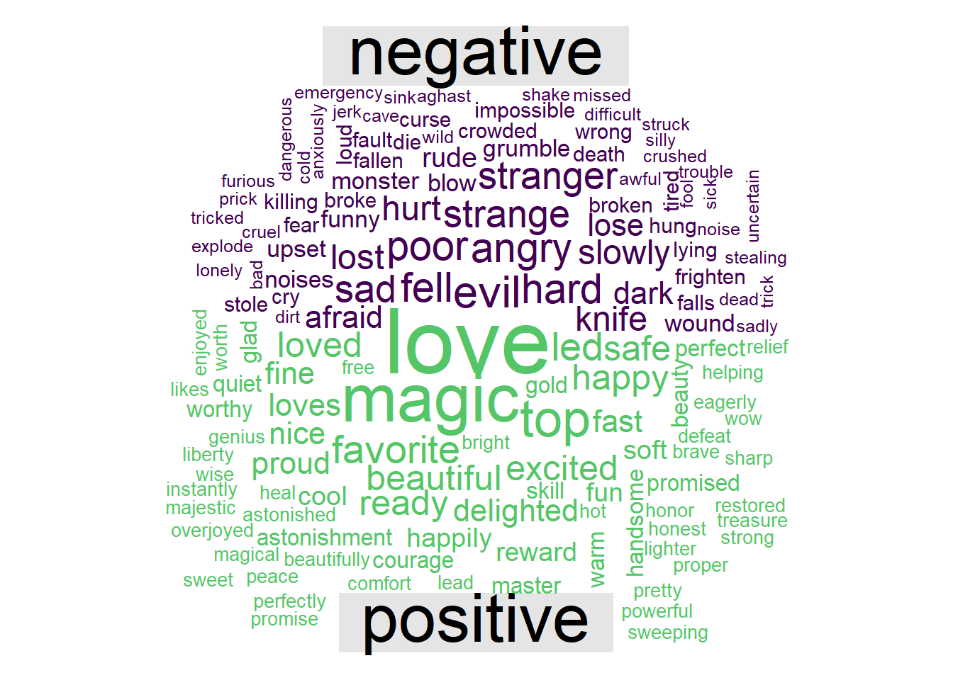
Figure 1: Wordcloud of positive and negative sentiment words
Immediately “love” and “magic” come forward as common words with positive sentiments. Some of the negative sentiment words look a bit ominous, and I question what I’m reading to my five-year-old; “die,” “killing,” “death,” and “knife” all make this list.
The question we sought to answer is: “Do books differ in sentiment depending on the gender of the main character?”
Because we will want to see this for the set of books and for the overall exposure, we will create a table that will include the count of times read, and then multiply the count of times read by the count of words to a get a weighted count of words.
gender_word_counts <- gender_tokens %>%
  inner_join(get_sentiments("bing")) %>%
  count(count, title, main_gender, word, sentiment, sort = TRUE) %>%
  mutate(n_weighted = n * count) %>%
  ungroup()
Before moving straight to the aggregate by gender of the main character, we should look at the sentiment scores for each book. Here I would like to note that the sentiment scores work best for short texts. Long texts that have many positive and many negative words often balance each other out with a total score near 0. Despite this, we can still use these sentiments to get a snapshot of the book.
For each book title, the table will include the number of sentiment words and the sentiment total (positive numbers mean more positive words, negative numbers mean more negative numbers).
gender_sentiment_summary <- gender_word_counts %>%
  group_by(count, title, main_gender, sentiment)
gender_sentiment_summary$sentiment_value <- gender_sentiment_summary$n
gender_sentiment_summary$sentiment_value[gender_sentiment_summary$sentiment == "negative"] <- -(gender_sentiment_summary$n)
gender_sentiment_summary %>%
  group_by(count, title, main_gender) %>%
  summarise(sentiment_count = sum(n), sentiment_total = sum(sentiment_value)) %>%
  arrange(-sentiment_total) %>%
  knitr::kable()
| count | title | main_gender | sentiment_count | sentiment_total |
|---|---|---|---|---|
| 2 | The Word Collector | Male | 29 | 15 |
| 4 | Bunheads | Female | 49 | 13 |
| 1 | Dear Girl | Female | 18 | 6 |
| 2 | The Wall in the Middle of the Book | Male | 6 | 4 |
| 4 | Flying High The Story of Gymnastics Champion Simone Biles | Female | 36 | 4 |
| 1 | Celtic Tales - The Kildare Pooka | Male | 38 | 3 |
| 1 | From My Window | Male | 10 | 2 |
| 1 | Wishes | Female | 4 | 2 |
| 1 | The Little Mermaid | Female | 17 | 1 |
| 2 | Moana | Female | 25 | 1 |
| 2 | Madeline’s Rescue | Female | 28 | 0 |
| 2 | Tangled Outside my Window | Female | 22 | 0 |
| 1 | Frozen - Look and Find | Female | 11 | -2 |
| 1 | Frozen | Female | 38 | -4 |
| 1 | The Hello, Goodbye Window | Female | 24 | -5 |
| 1 | The World Needs More Purple People | Female | 32 | -6 |
| 1 | Caps for Sale | Male | 18 | -10 |
| 1 | Sleeping Beauty | Female | 79 | -18 |
| 2 | My Mouth is a Volcano | Male | 35 | -23 |
| 1 | Caps for Sale and the Mindful Monkeys | Male | 24 | -25 |
| 1 | Celtic Tales - The Giant’s Stairs | Male | 114 | -44 |
| 2 | Celtic Tales - The Seal Catcher and the Selkies | Male | 127 | -45 |
The sentiment scores range from -56 to +17. At first glance, the books with female main characters appear more frequently on the positive half of the list and books with male main characters appear more frequently on the negative half of the list. Those at the very bottom are not surprising as they are mythology stories that are aimed for slightly older audiences.
Finally, let’s look at the sentiment scores aggregated by gender by grouping our results by the gender of the main character. We will also add a column for the weighted sentiment score which will multiple the books sentiment score by the number of times the book was read.
gender_summary <- gender_sentiment_summary %>%
  group_by(main_gender) %>%
  summarise(sentiment_total = sum(sentiment_value)) %>%
  arrange(-sentiment_total)

gender_summary_weighted <- gender_sentiment_summary %>%
  group_by(main_gender) %>%
  summarise(weighted_sentiment_total = sum(count * sentiment_value)) %>%
  arrange(-weighted_sentiment_total)

left_join(gender_summary, gender_summary_weighted) %>%
  knitr::kable()
| main_gender | sentiment_total | weighted_sentiment_total |
|---|---|---|
| Female | -8 | 44 |
| Male | -123 | -172 |
Books that feature female main characters have a sentiment score of -8, while books featuring male main characters have a sentiment score of -123. This is larger gap than I expected! Both are negative overall, but books with male main characters are much more negative.
Overall, books we read with male main characters featured more negative sentiment words.
When factoring in the number of times the books were read, this gap widens. The weighted sentiment score for books with female main character is +44, while the weighted sentiment score for books with male main characters drops to -172.
When choosing which books to re-read, our daughter tended to choose female-led books with more positive words and male-led books with more negative words.
The last part of our sentiment analysis will be to look at which words are contributing most to these sentiment scores. We will filter our previous results by gender of the main character and by the words used more frequently, find the sum of each sentiment word. Before creating the graph, we can change our counts of negative sentiment words to a negative number by using mutate(n = ifelse(sentiment == “negative,” -n, n)).
female_counts <- gender_word_counts %>%
  filter(main_gender %in% c("Female") & n > 2)
female_sums <- female_counts %>%
  group_by(word) %>%
  summarise(sum_n = sum(n)) %>%
  ungroup()
left_join(female_counts, female_sums) %>%
  mutate(n = ifelse(sentiment == "negative", -n, n)) %>%
  mutate(sum_n = ifelse(sentiment == "negative", -sum_n, sum_n)) %>%
  ggplot(aes(n, reorder(word, sum_n), fill = sentiment)) +
  geom_col(show.legend = FALSE) +
  facet_wrap(~main_gender, scales = "free_y") +
  labs(x = "Contribution to sentiment",
       y = NULL)
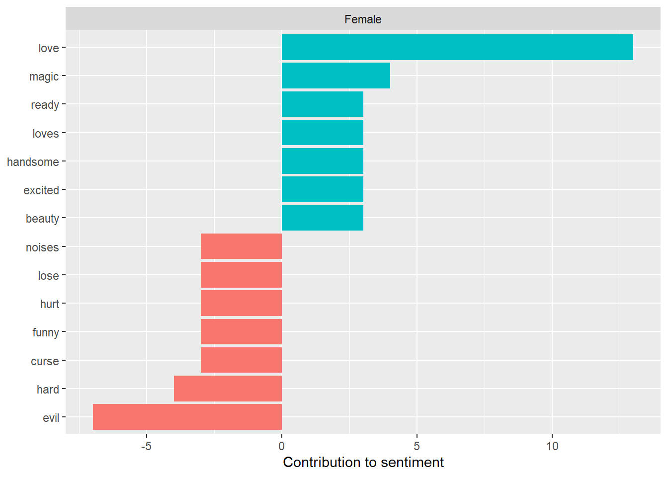
Figure 2: Highest Contributing Sentiment Words of Female Main Character Books
In this example, “love” is positive word contributing the most to the sentiment score of female-led books, while “evil” is the negative word contributing the most. These reflect the infiltration of Disney in our book selections - Rapunzel, The Little Mermaid, Frozen, Snow White all deal with love and evil (a reflection on that fact is for another time and place!).
We can use the same method for books with male main characters.
male_counts <- gender_word_counts %>%
  filter(main_gender %in% c("Male") & n > 2)
male_sums <- male_counts %>%
  group_by(word) %>%
  summarise(sum_n = sum(n)) %>%
  ungroup()
left_join(male_counts, male_sums) %>%
  mutate(n = ifelse(sentiment == "negative", -n, n)) %>%
  mutate(sum_n = ifelse(sentiment == "negative", -sum_n, sum_n)) %>%
  ggplot(aes(n, reorder(word, sum_n), fill = sentiment)) +
  geom_col(show.legend = FALSE) +
  facet_wrap(~main_gender, scales = "free_y") +
  labs(x = "Contribution to sentiment",
       y = NULL)
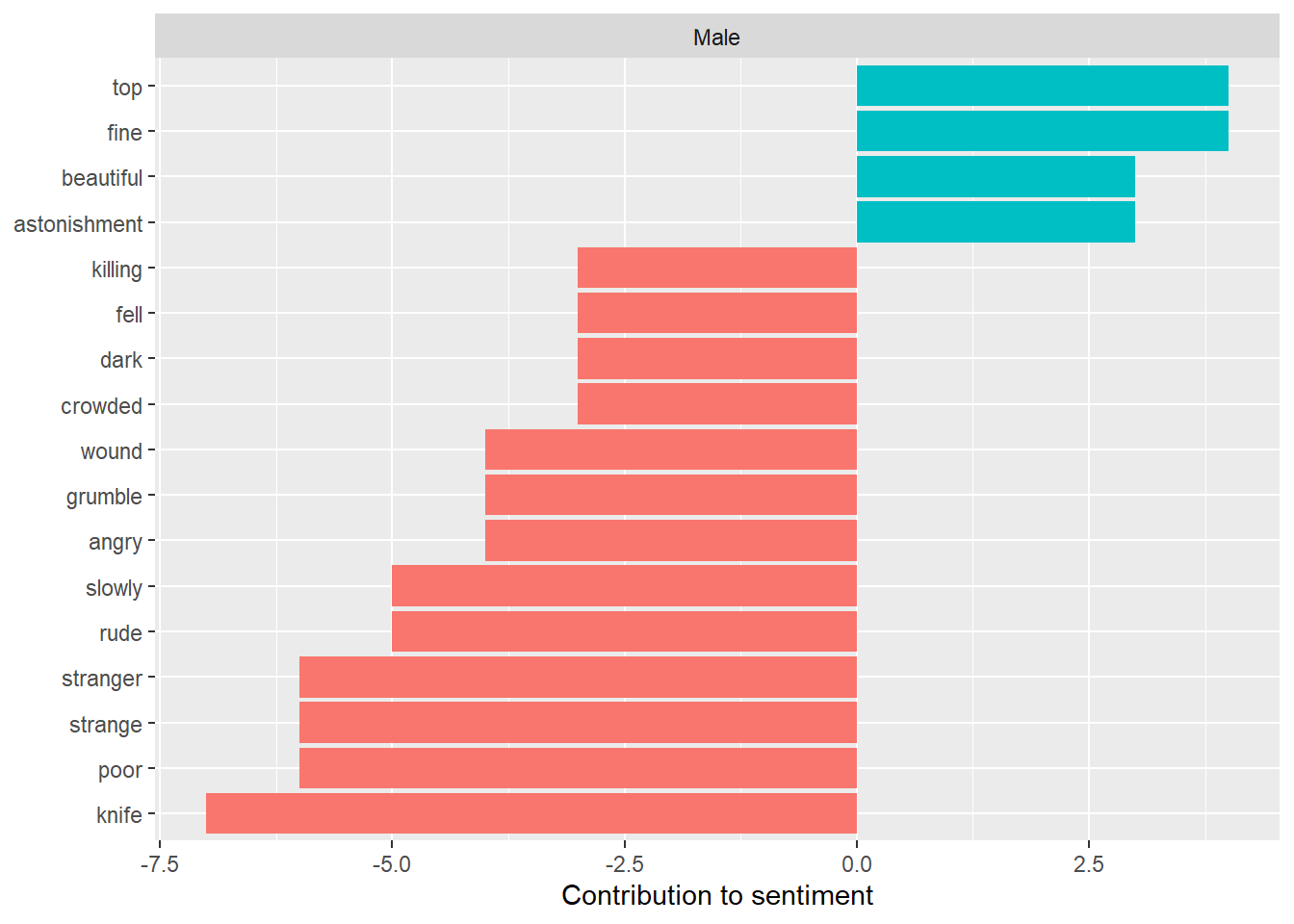
Figure 3: Highest Contributing Sentiment Words of Male Main Character Books
We can already see more negative words on this list - “knife,” “poor,” “strange,” to name the most contributing words. And some other dark entries, like “killing.”
Lastly, we can do the same, but based on exposure, by weighted the numbers by number of times the books were read.
female_weighted_sums <- female_counts %>%
  group_by(word) %>%
  summarise(sum_weighted = sum(n_weighted)) %>%
  ungroup()
left_join(female_counts, female_weighted_sums) %>%
  mutate(sum_weighted = ifelse(sentiment == "negative", -sum_weighted, sum_weighted)) %>%
  mutate(n_weighted = ifelse(sentiment == "negative", -n_weighted, n_weighted)) %>%
  ggplot(aes(n_weighted, reorder(word, sum_weighted), fill = sentiment)) +
  geom_col(show.legend = FALSE) +
  facet_wrap(~main_gender, scales = "free_y") +
  labs(x = "Contribution to sentiment",
       y = NULL)
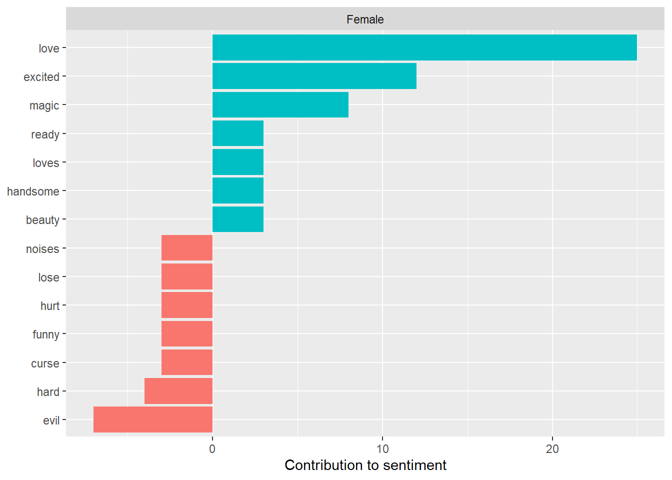
Figure 4: Highest Contributing Sentiment Words of Female Main Character Books by Exposure
“Love” pulls ahead even more! Our daughter tends to chose to read books that talk about love more than once.
male_weighted_sums <- male_counts %>%
  group_by(word) %>%
  summarise(sum_weighted = sum(n_weighted)) %>%
  ungroup()
left_join(male_counts, male_weighted_sums) %>%
  mutate(sum_weighted = ifelse(sentiment == "negative", -sum_weighted, sum_weighted)) %>%
  mutate(n_weighted = ifelse(sentiment == "negative", -n_weighted, n_weighted)) %>%
  ggplot(aes(n_weighted, reorder(word, sum_weighted), fill = sentiment)) +
  geom_col(show.legend = FALSE) +
  facet_wrap(~main_gender, scales = "free_y") +
  labs(x = "Contribution to sentiment",
       y = NULL)
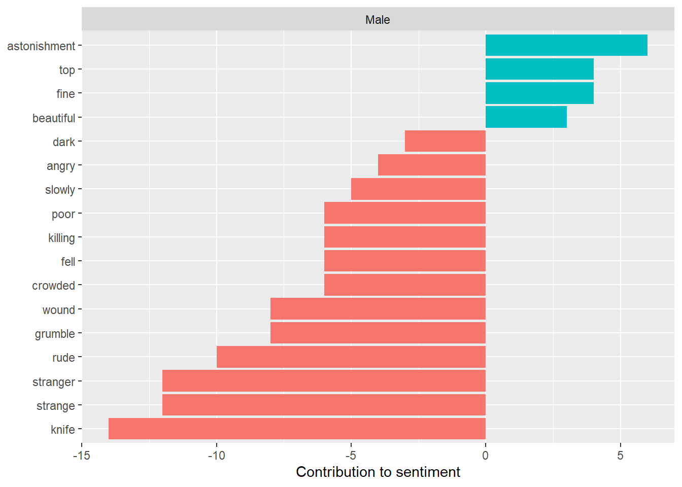
Figure 5: Highest Contributing Sentiment Words of Male Main Character Books by Exposure
There is not much change in the words contributing the sentiment score of books with male main characters, though the frequent words such as “knife” and “strange” had a higher contribution, again because these words were in books that were read more than once.
Summary
While only covering 15 days, our sample still contained 43 books over 68 reading sessions - much more than I anticipated! While I was happy to see these numbers, and to see the female representation in the books, there is still a lack of diversity in the main characters. There are two future actions that come to mind: (1) make sure more diversity is represented on her bookshelf by providing her with these books, and (2) encourage her to read these books, while still leaving the decision of which books to read to her.
The sentiment scores each individual book aligned with my views of the books, but when aggregated by gender of the main character, I was surprised to see the stark difference between the sentiments of books with female and male main characters. Not only did male-led books have a much lower sentiment score (-123, compared to -8 for female-led books), but this difference was made even greater when considering the number of times the books were read (-172 for male-led books, +44 for female-led books). Our daughter was choosing to re-read positive sentiment female-led books and negative sentiment male-led books.
As parents, we need to be conscious of what we are reading to our children, and how it portrays people who are similar and different to us. How are we filling the space around our children and what media are we providing them that will shape their view of the world?
Future Explorations
This is only scratching the surface. There were many more types of analyses I wanted to include, but had to cut short due to space. Some areas of future exploration:
- Analyze sentiment scores over the course of each book. A book with a neutral score might have few sentiment words, or it may start positive, turn negative as conflict grows, and return to positive when the conflict is resolved. Are there patterns for sentiments in these books?
- Look beyond the sentiment words, and more closely examine the relative word frequency by gender. I began doing this, but realized it went beyond the scope of this post.
- Clean up some of the repetitive code.
-
For more information on this package, see https://gt.rstudio.com/. ↩︎
-
While I love this package, there is a shortcoming in the inability to use table footnotes in R markdown. I will be looking to future workarounds for this. ↩︎